The Brownian Bridge Joint Max Position Distribution
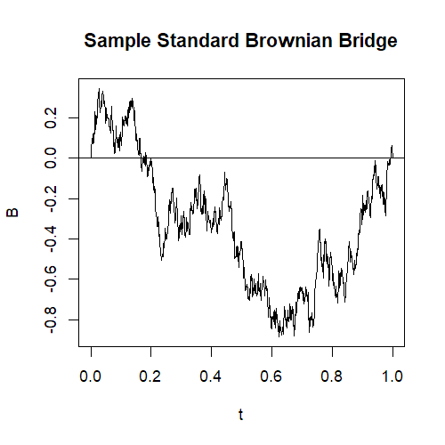
The standard Brownian bridge is a Wiener process from time 0 to 1 conditioned such that its value at time 1 is 0. Below is a sample path

Let $B_t, 0 \leq t \leq 1$ denote a standard Brownian bridge. It can be expressed in terms of the Wiener process:
\[B_t = W_t - t W_1\]From this one could derive the following properties using the independent Gaussian increments property of $W_t$.
- $\Expect(B_t) = 0$
- $\Cov(B_s, B_t) = \min(s, t) - s t$
There is one particular quantity of the Brownian bridge that is used commonly in statistics – its maximum value $M = \max_{0 \leq t \leq 1} B_t$. The distribution of this random variable is the asymptotic distribution of the test statistics in the CUSUM and Kolmogorov-Smirnov tests (more on this later).
The distribution of $M$ can be derived as follows. The strategy is to first get the joint density of the running maximum and current value of a Wiener process and condition on the current value at 1 being 0 to get the standard Brownian bridge.
To get the joint density, we first define $T_a = \inf {t \geq 0 : W_t = a}$ to be the first time that $W_t$ hits level $a$ and note that for $a \geq 0$ the event ${T_a \leq t}$ is equivalent to ${\max_{0 \leq s \leq t} W_s \geq a}$; in other words the process hitting $a$ before time $t$ happens if and only if its running maximum before $t$ is greater than or equal to $a$. Using the reflection principle,
\[\begin{align} \Prb( \max_{0 \leq s \leq t} W_s \geq a, W_t \leq x) &= \Prb(T_a \leq t, W_t \leq x) \\ &= \Prb(T_a \leq t, 2a - x \leq W_t) \\ &= \Prb(2a - x \leq W_t) \\ &= 1 - \Phi\left( \frac{2a - x}{\sqrt{t}} \right) \\ \Prb( \max_{0 \leq s \leq t} W_s \geq a, W_t \in \diff x) &= \frac{1}{\sqrt{2 \pi t}} \exp \left( \frac{- (2a - x)^2}{2t} \right) \diff x \\ \Prb( \max_{0 \leq s \leq 1} W_s \geq a | W_1 = 0 ) &= \frac{\frac{1}{\sqrt{2 \pi}} \exp(- 2a^2) \diff x}{\Prb(W_1 \in \diff x (0))} \\ &= \exp(- 2 a^2) \\ \Prb( \max_{0 \leq s \leq 1} W_s \in \diff a ) &= 4a \exp(- 2 a^2) \end{align}\]This is called a Rayleigh distribution and its pdf is plotted below. In addition, Beghin and Orsingher 1999 derive the general case of the distribution of the maximum of a Wiener process at any time $t$ when conditioned so that $W_u = \eta$ for any $u > 0$ and $\eta \in \R$.

Less well-known is the distribution of the time at which $B_t$ attains its maximum. As it happens, the maximal position has a uniform distribution on $[0, 1]$. Here is a proof, which uses the fact that a Brownian bridge cyclically translated an arbitrary $k \in [0, 1)$ length is still a standard Brownian bridge which has the same distribution of maximal position.
Joint density of maximum and position
We simulate 1000 standard Brownian bridges and plot all their maxima and maximal positions together.

As the figure shows, maxima attained near the middle are far higher than maxima attained near the ends, since bridge near the endpoints is pinned down to 0. The density of the joint distribution is
\[p(a, t) = \sqrt{\frac{2}{\pi}} \frac{a^2}{\big(t (1-t)\big)^\frac{3}{2}} \exp \left(- \frac{a^2}{2 t (1-t)} \right)\]This is readily obtained by conditioning on the joint density of $M_t$, $T_m$, and $W_t$ derived on page 101 of Karatzas and Shreve, Brownian Motion and Stochastic Calculus.
Improving hypothesis tests
As mentioned above, the joint distribution of maximum and position can be used to improve the power of hypothesis tests that use the Brownian bridge for the null distribution.
Simulations
« The Regularized Plackett-Luce Ranking Model
Variance Estimation in a Simple Kalman Filter »